これは単なる備忘録です。「論文とサンプルコード読みながら試しました」以外に何も内容のない記事ですのでご注意ください。特に個々の式の変数の説明については個人的な備忘録ゆえ大半を端折りますので、仮に興味を持たれた方は適宜論文の本文をご参照下さい。読んだ論文はこちら。
なお、この記事を書くに当たってid:ushi-goroshiさんのこちらのブログ記事シリーズを参考にさせていただきました。分かりやすくて大変助かりました、有難うございます。
それでは適当にやっていきます。
Ads carryover & shape effectsについて
いわゆるMedia Mix Modeling (MMM)の肝は「広告が投下されるとKPIが増える」というシンプルな市場反応構造の想定です。しかしながら、広告というものの性質を考えるとそれほどシンプルではなさそうだということが考えられます。理由は簡単で、
- 広告は数日・数週間・数ヶ月のスパンで人々の記憶に残る
- 広告の効果はどこかで飽和する
ということが経験則的に言えるからです。これらを勘案した上で回帰モデルを組むことで、実態としての市場反応により正確に沿ったMMMを推定できるということが期待されます。
そこで、この2つを適切にモデリングすることを考えます。前者は"Ad stock / carryover"効果と呼ばれ、ある程度のタイムラグを置いても広告の効果が市場反応に現れるという性質を表すものです。論文中では以下の式で定義しています。
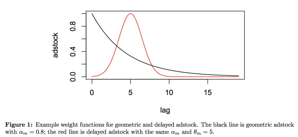
この式に従ってcarryover functionを描画したものがFigure 1です。次に後者は薬理学分野で使われる"Hill"関数を用いてモデリングします。これは広告の投下量に従って飽和したり、あるいは効果が伸び続けるという効果を表します。論文中では以下の式で定義しています。

この式に従ってshape functionを描画したものがFigure 2です。この2つの式と、広告以外の操作変数による効果を合わせたものが式(7)として示されています。
これが最終的なMMMのモデル式であり、これに事前分布を含めたチューニングパラメータを与えてやり、を推定するというのがここでの目標です。なお得られた
からROAS即ち投資効率を推定するのはまた別の話なので、ここでは一旦割愛します。
RStanでパラメータ推定までやってみる
やるべきことは非常に簡単です。まず論文中のStanコードを写経します。'shape_carryover_mmm.stan'などと名付けておきます。
# 'shape_carryover_mmm.stan'
functions {
  // the Hill function
  real Hill(real t, real ec, real slope) {
    return 1 / (1 + (t / ec)^(-slope));
  }
  // the adstock transformation with a vector of weights
  real Adstock(row_vector t, row_vector weights) {
    return dot_product(t, weights) / sum(weights);
  }
}

data {
  // the total number of observations
  int<lower=1> N;
  // the vector of sales
  real<lower=0> Y[N];
  // the maximum duration of lag effect, in weeks
  int<lower=1> max_lag;
  // the number of media channels
  int<lower=1> num_media;
  // a vector of 0 to max_lag - 1
  row_vector[max_lag] lag_vec;
  // 3D array of media variables
  row_vector[max_lag] X_media[N, num_media];
  // the number of other control variables
  int<lower=1> num_ctrl;
  // a matrix of control variables
  row_vector[num_ctrl] X_ctrl[N];
}

parameters {
  // residual variance
  real<lower=0> noise_var;
  // the intercept
  real tau;
  // the coefficients for media variables
  vector<lower=0>[num_media] beta_medias;
  // coefficients for other control variables
  vector[num_ctrl] gamma_ctrl;
  // the retention rate and delay parameter for the adstock transformation of
  // each media
  vector<lower=0,upper=1>[num_media] retain_rate;
  vector<lower=0,upper=max_lag-1>[num_media] delay;
  // ec50 and slope for Hill function of each media
  vector<lower=0,upper=1>[num_media] ec;
  vector<lower=0>[num_media] slope;
}

transformed parameters {
  // a vector of the mean response
  real mu[N];
  // the cumulative media effect after adstock
  real cum_effect;
  // the cumulative media effect after adstock, and then Hill transformation
  row_vector[num_media] cum_effects_hill[N];
  row_vector[max_lag] lag_weights;
  for (nn in 1:N) {
    for (media in 1 : num_media) {
      for (lag in 1 : max_lag) {
        lag_weights[lag] = pow(retain_rate[media], (lag - 1 - delay[media]) ^ 2);
      }
      cum_effect = Adstock(X_media[nn, media], lag_weights);
      cum_effects_hill[nn, media] = Hill(cum_effect, ec[media], slope[media]);
    }
    mu[nn] = tau +
      dot_product(cum_effects_hill[nn], beta_medias) +
      dot_product(X_ctrl[nn], gamma_ctrl);
  }
}

model {
  retain_rate ~ beta(3,3);
  delay ~ uniform(0, max_lag - 1);
  slope ~ gamma(3, 1);
  ec ~ beta(2,2);
  tau ~ normal(0, 5);
    for (media_index in 1 : num_media) {
      beta_medias[media_index] ~ normal(0, 1);
    }
    for (ctrl_index in 1 : num_ctrl) {
      gamma_ctrl[ctrl_index] ~ normal(0,1);
    }
    noise_var ~ inv_gamma(0.05, 0.05 * 0.01);
    Y ~ normal(mu, sqrt(noise_var));
}
次に、論文を読みながらAdstock関数とHill関数を設定します。
Adstock <- function(t, weights){
  (t %*% weights) / sum(weights)
}

Hill <- function(t, ec, slope){
  1 / (1 + (t / ec)^(-slope))
}
最後に、Stanコードを参考に逆にシミュレーションデータを生成するR関数を書きます。
Generate_y <- function(X_media, X_ctrl, N, num_media, max_lag, retain_rate, delay, ec, slope, beta_medias, gamma_ctrl, tau, noise_sd){
  # X_media: N * num_media * (max_lag), should be normalized to [0, 1]
  # X_ctrl: N * num_ctrl
  # N: nrow(X)
  # num_media: ncol(X)
  # max_lag: just specify
  # retain_rate: 0 ~ 1, vector[num_media]
  # delay: 0 ~ (max_lag-1), vector[num_media]
  # ec: 0 ~ 1, vector[num_media]
  # slope: 0~, vector[num_media]
  # beta_medias: 0 ~
  # gamma_ctrl: as you like it (just dummy variables)
  # tau: intercept, as you like it
  # noise_sd: SD of normal distribution noise for Y, as you like it
  mu <- rep(0, N)
  lag_weights <- rep(0, max_lag)
  cum_effects_hill <- matrix(0, nrow = N, ncol = num_media)
  for (nn in 1:N){
    for (media in 1:num_media){
      for (lag in 1:max_lag){
        lag_weights[lag] <- retain_rate[media]^((lag - 1 - delay[media])^2)
      }
      cum_effect <- Adstock(X_media[nn, media, ], lag_weights)
      cum_effects_hill[nn, media] <- Hill(as.numeric(cum_effect), ec[media], slope[media])
    }
    mu[nn] <- tau + cum_effects_hill[nn, ] %*% beta_medias + X_ctrl[nn, ] %*% gamma_ctrl
    + rnorm(1, 0, noise_sd)
  }
  return(mu)
}
ただしこのままだと式の形を見れば分かるようにきちんと正規分布ノイズが乗らないので、最後の最後に以下のようにして補正します。
Y <- Y + rnorm(N, 0, noise_sd)
あとは単に各種パラメータを設定して実行するだけです。今回はこんな感じのパラメータを与えてやってみます。
> set.seed(111)
> X <- runif(300, 0, 1)
> X_media <- array(0, c(100, 3, 5))
> for (i in 1:3){
+ X_media[,,i] <- X
+ }
> set.seed(112)
> X_ctrl <- matrix(round(runif(200, 0, 0.65)), nrow = 100, ncol = 2)
> N <- 100
> num_media <- 3
> max_lag <- 5
> retain_rate <- c(0.5, 0.1, 0.3)
> delay <- 0:4
> ec <- c(0.1, 0.2, 0.1)
> slope <- c(0.05, 0.1, 0.15)
> beta_medias <- c(0.4, 0.6, 0.2)
> gamma_ctrl <- c(0.005, 0.01)
> tau <- 0.5
> noise_sd <- 0.05
> Y <- Generate_y(X_media, X_ctrl, N, num_media, max_lag, retain_rate, delay, ec, slope, beta_medias, gamma_ctrl, tau, noise_sd)
> set.seed(113)
> Y <- Y + rnorm(N, 0, noise_sd)
> plot(Y, type = 'l')
> dat <- list(N = N, Y = Y, X_media = X_media, num_media = num_media, max_lag = max_lag, num_ctrl = 2, X_ctrl = X_ctrl, lag_vec = 0:(max_lag-1))
> library(rstan)
> options(mc.cores = parallel::detectCores())
> rstan_options(auto_write = TRUE)
> fit <- stan('shape_carryover_mmm.stan', data = dat, iter = 1000, chains = 4)
結果はこんな感じになります。
> options(max.print = 10000)
> fit
Inference for Stan model: amt_mmm.
4 chains, each with iter=1000; warmup=500; thin=1;
post-warmup draws per chain=500, total post-warmup draws=2000.

                          mean se_mean   sd   2.5%    25%    50%    75%  97.5% n_eff Rhat
noise_var                 0.00    0.00 0.00   0.00   0.00   0.00   0.00   0.00  1631 1.00
tau                       1.05    0.01 0.06   0.84   1.04   1.07   1.09   1.11    79 1.07
beta_medias[1]            0.51    0.02 0.56   0.01   0.06   0.32   0.78   1.98  1128 1.00
beta_medias[2]            0.30    0.01 0.37   0.03   0.09   0.17   0.34   1.41   743 1.01
beta_medias[3]            0.47    0.02 0.53   0.01   0.07   0.28   0.72   1.88   615 1.00
gamma_ctrl[1]             0.01    0.00 0.01  -0.02   0.00   0.01   0.02   0.03  2000 1.00
gamma_ctrl[2]             0.03    0.00 0.01   0.00   0.02   0.03   0.04   0.05  1798 1.00
retain_rate[1]            0.45    0.00 0.18   0.13   0.32   0.45   0.57   0.80  1510 1.00
retain_rate[2]            0.50    0.00 0.19   0.17   0.36   0.50   0.64   0.86  2000 1.00
retain_rate[3]            0.48    0.00 0.18   0.14   0.35   0.48   0.61   0.84  2000 1.00
delay[1]                  3.10    0.04 0.93   0.39   2.89   3.40   3.74   3.97   513 1.00
delay[2]                  2.13    0.04 1.17   0.10   1.08   2.28   3.16   3.89   794 1.01
delay[3]                  2.88    0.05 1.02   0.23   2.56   3.20   3.60   3.95   507 1.01
ec[1]                     0.57    0.00 0.21   0.15   0.41   0.59   0.74   0.92  2000 1.00
ec[2]                     0.52    0.01 0.22   0.13   0.34   0.52   0.70   0.92  1047 1.00
ec[3]                     0.57    0.01 0.22   0.12   0.41   0.58   0.73   0.92  1683 1.00
slope[1]                  3.25    0.04 1.73   0.82   1.95   2.97   4.25   7.40  1632 1.00
slope[2]                  1.73    0.06 1.26   0.21   0.84   1.44   2.27   4.82   440 1.00
slope[3]                  2.94    0.05 1.66   0.53   1.70   2.74   3.82   7.05  1217 1.00
mu[1]                     1.13    0.00 0.01   1.11   1.13   1.13   1.14   1.15  1148 1.00
mu[2]                     1.12    0.00 0.02   1.09   1.11   1.12   1.13   1.15  1375 1.00
mu[3]                     1.14    0.00 0.02   1.11   1.13   1.14   1.15   1.17  1625 1.00
# 中略 #
mu[98]                    1.16    0.00 0.01   1.14   1.15   1.16   1.17   1.19  1636 1.00
mu[99]                    1.12    0.00 0.02   1.08   1.10   1.11   1.13   1.15  1221 1.00
mu[100]                   1.15    0.00 0.01   1.13   1.14   1.15   1.16   1.18  1347 1.00
cum_effect                0.27    0.01 0.26   0.01   0.07   0.17   0.39   0.81   444 1.01
cum_effects_hill[1,1]     0.10    0.01 0.21   0.00   0.00   0.00   0.06   0.77   485 1.00
cum_effects_hill[1,2]     0.36    0.01 0.25   0.01   0.11   0.37   0.52   0.90   635 1.01
cum_effects_hill[1,3]     0.17    0.01 0.26   0.00   0.00   0.03   0.27   0.87   317 1.01
# 中略 #
cum_effects_hill[100,1]   0.14    0.01 0.25   0.00   0.00   0.01   0.12   0.88   448 1.00
cum_effects_hill[100,2]   0.46    0.01 0.28   0.02   0.20   0.50   0.65   0.97   612 1.01
cum_effects_hill[100,3]   0.19    0.02 0.27   0.00   0.01   0.04   0.32   0.91   319 1.01
lag_weights[1]            0.12    0.01 0.26   0.00   0.00   0.00   0.05   0.97   772 1.01
lag_weights[2]            0.21    0.01 0.32   0.00   0.00   0.04   0.29   0.99   598 1.00
lag_weights[3]            0.39    0.01 0.30   0.01   0.13   0.31   0.61   0.99   739 1.01
lag_weights[4]            0.69    0.01 0.31   0.00   0.54   0.81   0.95   1.00   471 1.00
lag_weights[5]            0.56    0.01 0.36   0.00   0.22   0.64   0.90   1.00   589 1.01
lp__                    205.39    0.17 3.69 197.59 202.96 205.63 208.02 211.88   479 1.01

Samples were drawn using NUTS(diag_e) at Sat Sep  1 16:53:22 2018.
For each parameter, n_eff is a crude measure of effective sample size,
and Rhat is the potential scale reduction factor on split chains (at
convergence, Rhat=1).
> stan_dens(fit, pars = 'lp__')
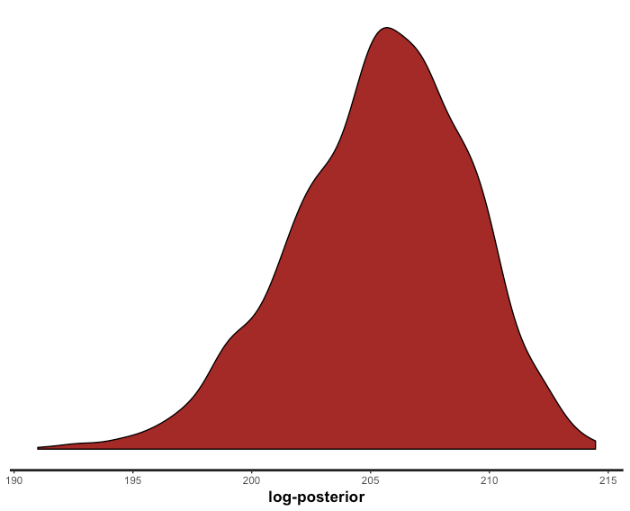
そんなに極端にMCMCサンプリングの収束は悪くないことが分かります。では、即ち時系列の当てはめ値を出して、本来のYと比べてみます。
> stan_dens(fit, pars = 'lp__')
> efit <- extract(fit)
> mu <- rep(0, N)
> for (i in 1:N){
+ tmp <- density(efit$mu[,i])
+ mu[i] <- tmp$x[tmp$y == max(tmp$y)]
+ }
> matplot(cbind(Y, mu), type = 'l', lty = 1)
> cor(Y, mu)
[1] 0.4272222
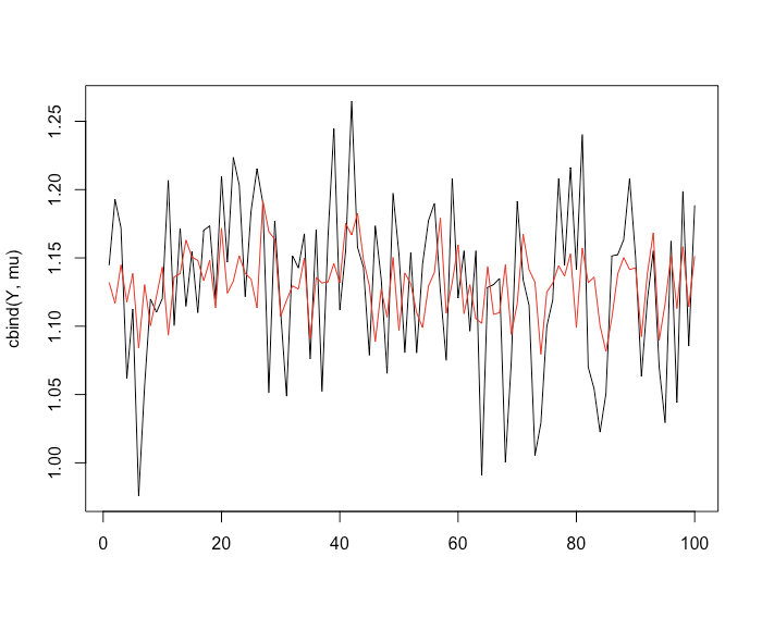
うーん、当てはまっているような当てはまっていないような。。。パラメータ推定もあまり当たっていない気がします。事前分布の与え方が良くないのかもしれません。ちょっとまた色々検討してみます。
追記
この記事の1年後ぐらいに非常に優れた解説記事が出ていました。
この記事の3年後ぐらいに、さらに優れた解説&検証資料が出ていました。